Mastering Pivot Tables in Excel: A Guide to Simplifying Data Analysis
Pivot tables in Microsoft Excel are a powerful feature that allows users to summarize and analyze large datasets in a user-friendly manner. By organizing and consolidating data, pivot tables enable you to extract meaningful information and identify trends that might not be immediately apparent.
Understanding Pivot Tables A pivot table is essentially a data summarization tool that can sort, count, total, or average data stored in one table or spreadsheet. It displays the results in a second table (the pivot table) without altering the original data. This makes pivot tables particularly useful for quickly creating reports from complex data.
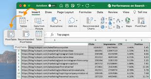
Creating a Pivot Table To create a pivot table:
- Click on any single cell within your dataset.
- Navigate to the Insert tab and select PivotTable.
- Excel will automatically select the data for the pivot table and suggest a new worksheet as its location.
- Click OK, and the PivotTable Fields pane will appear.
- Organizing Data With the PivotTable Fields pane, you can drag and drop fields into different areas to organize your data:
Pivot Table Features
Rows Area: Displays the rows of your pivot table.
Columns Area: Displays the columns of your pivot table.
Values Area: Contains the data to be summarized.
Filters Area: Allows you to filter the data that is included in your pivot table.
Process Of Analyzing Data On Pivot Table
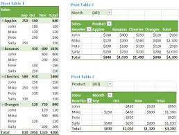
Analyzing Data Once your pivot table is set up, you can start analyzing your data. For instance, if you want to see the total sales for each product category:
Drag the Product Category field to the Rows area.
Drag the Sales field to the Values area.
Use the Filters area to include or exclude certain data points.
Sorting and Filtering Pivot tables allow you to sort data in ascending or descending order. You can also apply filters to focus on specific segments of your data. For example, you could filter to view only sales data for a particular region or time period.
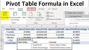
Changing Summary Calculation By default, Excel summarizes your data by summing or counting items. You can change this by:
Clicking any cell in the Values area.
Right-clicking and selecting Value Field Settings.
Choosing the type of calculation you want, such as average or count.
Refreshing Data If the original dataset changes, you can refresh your pivot table to reflect the updates. Simply right-click anywhere in the pivot table and select Refresh.
Conclusion
Pivot tables are an indispensable tool for anyone looking to make sense of large datasets in Excel. They offer a dynamic way to reorganize, summarize, and analyze data, making it easier to discover patterns and insights. With the ability to sort, filter, and calculate data in various ways, pivot tables provide a flexible solution for data analysis challenges. Whether you’re a business professional, researcher, or student, mastering pivot tables will undoubtedly enhance your data analysis capabilities and help you make more informed decisions based on your data.